Support Vector Machine

The Support Vector Machine (SVM) algorithm, a cornerstone in supervised machine learning, excels in solving complex classification and regression problems. Commonly known as support vector machines, these models are adept at handling diverse data types.

In the training phase, SVMs utilize a robust dataset comprising numerous examples. Each data point in the dataset is an example, represented by a feature vector x_i and an associated label.

$$ ( X , y ) $$

Here, X denotes a matrix consisting of vectors x_i, where each vector embodies the characteristics of an example and pinpoints a location in n-dimensional space. The vector y holds the labels, providing the correct classification for each data point.

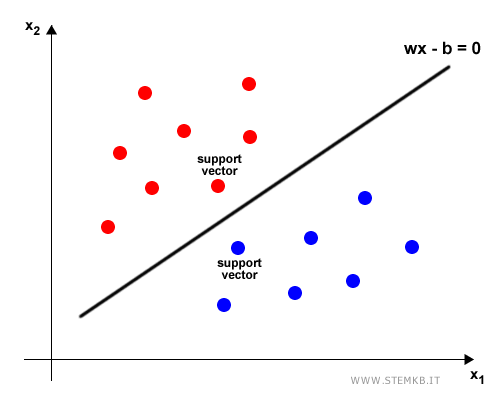
SVMs operate by identifying a hyperplane that effectively segregates the dataset into two distinct categories.

The critical separator, known as the decision boundary, delineates these categories.

Example. In a two-feature scenario, this hyperplane manifests as a line bisecting the dataset.

In three dimensions, the hyperplane becomes a plane. As the number of features increases beyond three, the hyperplane extends into a multi-dimensional construct.

Points nearest the hyperplane are more sensitive to new data introduction. A minor adjustment to the hyperplane can shift their classification, which is why these points are called support vectors.

Points farther from the hyperplane, however, are more likely to retain their correct classification status.

The term margin is used to describe the distance between the support vectors and the decision boundary.

Note. The margin is the gap between the planes defined by wx-b=1 and wx-b=-1. This gap measures 2/||w||. Therefore, minimizing the Euclidean norm ||w|| enlarges the margin, a key objective of the SVM algorithm.

A larger margin is synonymous with superior generalization capabilities, enhancing the algorithm's proficiency in classifying new data.

Thus, the effectiveness of SVM classification is directly proportional to the distance between the hyperplane and the support vectors.

The hyperplane itself is determined by the equation

$$ wx - b = 0 $$

Note. The vector w={w₁, w₂, ..., w_j} consists of j real numbers, each representing a weight corresponding to a feature x={x₁, x₂, ..., x_j} in the dataset. Thus, wx is a linear combination, typically in the form w₁x₁ + w₂x₂ + ... + w_jx_j.

Optimal values for w and b are determined through an optimization problem solved during the SVM's training phase.

Once these values are established, they are utilized in a sign function for data classification purposes.

$$ y = sign(w*x-b*) $$

y assumes the following values:

• +1 if the function w*x-b*≥0
• -1 if the function w*x-b*≤0

This functionality forms the crux of the SVM's statistical model.

Note. In simpler models, the decision boundary is linear, appearing as either a straight line or plane that divides the dataset. However, in more advanced models, this boundary can be nonlinear, taking on a curved shape.