Probability distributions of random numbers in Matlab

In this lesson, I will explain how to use probability distributions to generate random numbers.

Why change distributions? Matlab allows you to generate random numbers using various probability distributions (exponential, normal, Poisson, gamma). The choice of distribution depends on what you want to simulate. Some real-world phenomena are better simulated with one distribution over another.

Let's look at some practical examples.

Generate a pseudorandom number using the rand() or randi() function

>> rand(1)

In these cases, Matlab uses the default uniform distribution where all values are uniformly distributed among all possible values.

For example, generate a 100x100 matrix with random values between 0 and 1 and assign it to the variable x

This command generates ten thousand random values.

>> x=rand(100);

Now visualize the distribution of values using a histogram with the hist() function

>> hist(x)

The random values you just generated are uniformly distributed between 0 and 1.

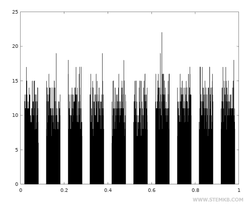
Note. In the plot, the horizontal axis indicates the random values from 0 to 1, which is the range of possible values. The vertical axis measures the frequency with which values repeat. The frequency is roughly the same for every value.

If you use other probability distributions, the result is very different.

The exponential distribution

To generate random numbers using the exponential distribution, you need to use the exprnd() function

>> exprnd(1)
ans = 0.90844

For example, type exprnd(1,3,2) to generate a 3x2 matrix with random values using the exponential distribution with a mean value of 1.

>> exprnd(1,3,2)
ans =
1.09340 0.28265
0.10781 1.72641
0.20653 0.87235

What changes compared to the uniform distribution?

To understand, generate a 100x100 random matrix using the exprnd() function

>> x=exprnd(1,100,100);

Then visualize the random values you just generated using a histogram of frequencies with the hist() function

>> hist(x)

In the exponential distribution, the random values are concentrated at the beginning of the range of possible values.

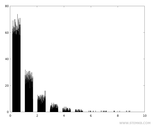
In this case, values close to zero or the initial value of the range are much more frequent.

The frequency decreases exponentially in higher values.

The normal distribution

To generate random numbers using the normal distribution, use the randn() function

>> randn(1)
ans = 0.85251

For example, type randn(2,3) to create a 2x3 random matrix

>> randn(2,3)
ans =
-0.32674 2.24641 -0.19528
-0.37856 0.13721 0.41417

Now generate a 100x100 matrix of random values using the normal distribution

>> x=randn(100);

Then visualize the histogram of frequencies of the random values using the hist() function

>> hist(x)

In the normal distribution, the most frequent values are centered within the range of possible values.

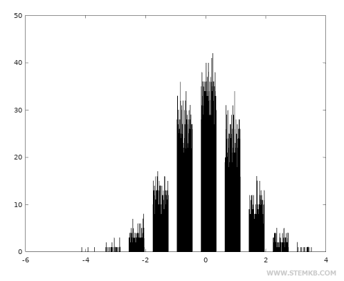
The frequency of random values decreases as you move away from zero, both to the right and to the left.

The Normal Distribution is characterized by a bell-shaped curve.

The Poisson Distribution

To generate random numbers with the Poisson Distribution, you can use the poissrnd() function.

>> poissrnd(1)
ans = 3

The Poisson Distribution generates random numbers around a mean value.

Example. When the parameter of the poissrnd(1) function is set to 1, it generates random numbers from a Poisson distribution with an average value of 1.

For example, you can type poissrnd(5,2,3) to create a 2x3 random matrix composed of values around the mean value of 5.

>> poissrnd(5,2,3)
ans =
3 7 6
5 2 2

You can also generate a 100x100 random matrix of values around the mean value of 5.

>> x=poissrnd(5,100,100)

Then, you can display the histogram of frequencies using the hist() function.

>> hist(x)

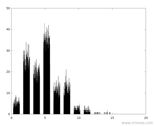
In the Poisson Distribution, random values are typically concentrated around the mean value of 5.

The Gamma Distribution

To generate random numbers using the Gamma Distribution, you can use the randg() command.

>> randg(1)
ans = 2.5621

For instance, you can type randg(100,2,3) to produce a 2x3 random matrix around the central value of 100.

>> randg(100,2,3)
ans =
101.843 98.346 87.956
93.809 99.350 93.122

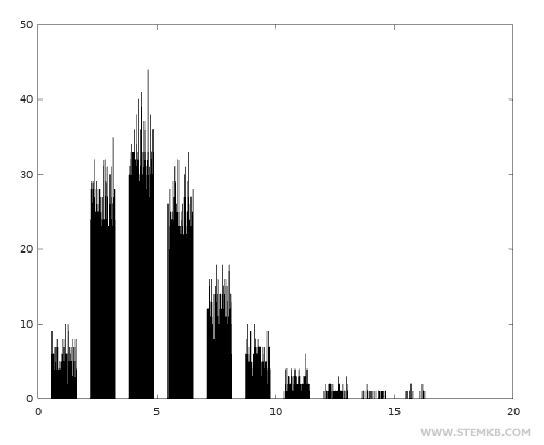
You can also generate a 100x100 random matrix with the Gamma Distribution around the central value of 5.

>> x = randg(5,100,100)

Then, you can display the histogram of frequencies using the hist() function.

>> hist(x)

In the Gamma Distribution, values close to the central value are more frequent.

By using these probability distributions in MATLAB, you can generate random numbers with various characteristics.

These functions can be used to generate single random values, vectors, or matrices composed of random values.