Exponential Function in Scilab

Within the Scilab environment, the exp() function stands out as a powerful tool, designed to compute the exponential of any number.

exp(x)

This isn't just any function—it's a core, built-in feature of Scilab.

When invoked, the function diligently returns the exponential of the number x. Whether you're working with a singular value or an array of numbers, exp() has you covered.

But what is the exponential function at its core? It's the representation of the number "e", the base of the natural logarithm (approximately 2.71828), raised to the power of x. In mathematical terms: $$ exp(x) = e^x $$

To illustrate its utility, consider this simple application.

To compute the exponential of 2 using exp():

exp(2)

The outcome? A value of approximately 7.389, representing e².

7.3890561

But the versatility of exp() doesn't end there. It seamlessly integrates with arrays, vectors, and matrices

Take, for instance, a vector A.

A = [1, 2, 3, 4];

Compute the exponential of each element in A.

exp(A)

Here, exp() meticulously calculates the exponential for each individual element, returning an array of identical dimensions.

2.7182818 7.3890561 20.085537 54.59815

In essence, the function is computing the results for exp(1), exp(2), exp(3), and exp(4).

It's worth noting that Scilab's mathematical constant %e can also be used to obtain the value of exp(1), which equates to the number "e" (e¹=2.7182818). While the results are consistent, the constant %e boasts superior efficiency, demanding fewer computational resources than its counterpart, exp(1).

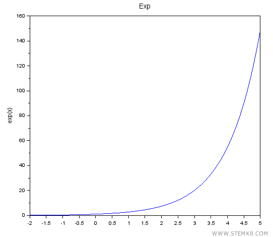
For those keen on visual representation, the following script can be employed to plot the function:

 

1. x = linspace(-2, 5, 1000);
2. y = exp(x);
3. plot(x, y);
4. xlabel('x');
5. ylabel('exp(x)');
6. title('Exp');

This visualization captures the essence of the exponential function, plotting its trajectory from -2 to 5.

A key takeaway? The exponential function maintains a positive trajectory, defined across all real numbers, spanning from -∞ to +∞.