The Cosine Function within Scilab

In Scilab, the cos() function serves as a powerful tool for computing the cosine of either a singular number or an array of numbers.

cos(x)

In this context, 'x' denotes the magnitude of an angle, expressed in radians.

The function, when executed, yields the cosine value corresponding to the given angle.

This is one of the integral trigonometric functions embedded within Scilab. Interestingly, the 'x' parameter is versatile; it can be a standalone value or an array of values.

Let's delve into a practical example.

To determine the cosine of π/4 (equivalent to 45°), employ the cos() function.

cos(%pi / 4)

Here, the symbol %pi represents Scilab's designated constant for the value of pi, which is approximately 3.14.

The outcome for the cosine of π/4 is 0.7071068.

0.7071068

Moreover, the function is adept at handling arrays.

Consider defining an array with three distinct values under the variable "v"

v = [0, %pi / 2, %pi]

Subsequently, compute its cosine:

cos(v)

In this instance, the cos() function processes and outputs an array, each entry representing the cosine of the respective element from the "v" array.

The results are:

1. 0 -1.

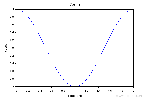
For those inclined towards a visual representation, Scilab's plotting capabilities come in handy.

To illustrate, the cosine function can be plotted as:

1. x = linspace(0, 2, 1000);
2. y = cos(x * %pi);
3. plot(x, y);
4. xlabel('x (radiant)');
5. ylabel('cos(x)');
6. title('Cosine');

Executing the above script will render a plot showcasing the cosine function spanning from 0 to 2π radians.