Mathematical Operations in Scilab

This tutorial gently guides you through basic mathematical operations that Scilab handles with ease. Let's delve into them.

Arithmetic Operations

Scilab allows seamless execution of fundamental arithmetic operations - be it addition, subtraction, multiplication, or division.

Simply input the operations using the arithmetic symbols +, -, *, /, and press Enter. Scilab takes care of the rest.

Adding Values

For summing two values, use the "+" operator.

--> 2 + 3
ans =
5

Subtracting Values

To find the difference between two numbers, deploy the "-" operator.

--> 7 - 4
ans =
3.

Multiplying Values

For the product of two values, the "*" operator comes in handy.

--> 3 * 4
ans =
12.

Dividing Values

For the quotient from a division operation, use the "/" operator.

--> 8 / 2
ans =
4.

Integer Division

Need to calculate integer division? Nest your division inside the int() function.

--> int(8 / 3)
ans =
2.

Calculating Remainder

Find out the remainder from division with the modulo(a,b) function.

--> modulo(8,3)
ans =
2.

Power

Raise a value to a power using the "^" operator.

--> 8^2
ans =
64.

Mathematical Operations: Order Matters

Scilab dutifully obeys the order of operations rule in mathematics.

1. Parentheses take priority in an expression.
2. For nested parentheses, Scilab starts from the innermost bracket, working its way out.
3. Then come powers and roots, followed by multiplications and divisions from left to right.
4. Lastly, additions and subtractions follow suit.

Precise use of parentheses helps to execute mathematical operations in your preferred sequence.

Ready-to-Use Mathematical Functions

Scilab comes loaded with several predefined mathematical functions including square root, trigonometric functions, and exponential and logarithmic functions.

Square Root

Tap into the sqrt() function to calculate the square root.

--> sqrt(9)
ans =
3.

Nth Root

Calculating the nth root of a number 'a'? Use the formula a^(1/n), where 'n' is the desired root's order.

For instance, to calculate the cubic root of 27, type 27^(1/3)

--> 27^(1/3)
ans =
3.

Exponential Function

The exp() function calculates the exponential function e^x.

--> exp(2)
ans =
7.3891

Logarithm

For the base 10 logarithm, the log10() function is your go-to tool.

--> log10(100)
ans =
2.

Natural Logarithm

For the natural logarithm (base "e"), simply use the log() function.

--> log(2.71)
ans =
0.9969486

Sine

To calculate the trigonometric function "sine", use the sin() function

--> sin(%pi / 4)
ans =
0.7071

Cosine

To calculate the trigonometric function "cosine", use the cos() function

--> cos(%pi / 3)
ans =
0.5

Tangent

To calculate the trigonometric function "tangent", use the tan() function

--> tan(%pi / 4)
ans =
1

Matrices and Matrix Operations

Creating a matrix in Scilab is simple with the following syntax:

--> A = [1, 2; 3, 4]
A =
1 2
3 4

Now also create a second matrix

--> B = [5, 6; 7, 8]
B =
5 6
7 8

You can easily perform various operations such as addition, subtraction, multiplication, and transpose on matrices.

Sum of Two Matrices

To add two matrices, use the "+" operator

--> A + B
ans =
6 8
10 12

Difference between Matrices

To obtain the difference between two matrices, use the "-" operator

--> A - B
ans =
-4 -4
-4 -4

Multiplication between Matrices

To multiply two matrices, use the "*" operator

--> A * B
ans =
19 22
43 50

Matrix Transposition

To obtain the transposed matrix, use the ' symbol after the matrix name.

--> A'
ans =
1 3
2 4

Inverse Matrix

To calculate the inverse matrix, use the inv() function

--> inv(A)
ans =
-2. 1.
1.5 -0,5

Solving Linear Equations

Scilab also has you covered when it comes to systems of linear equations, which you can solve using the linsolve() command.

For example, to solve the following system of linear equations:

$$ \begin{cases} x + 2y = 8 \\ \\ 3x - y = 5 \end{cases} $$

Firstly, create the coefficient matrix

--> A = [1, 2; 3, -1]
A =
1 2
3 -1

and the vector of the system's known terms

--> b = [8; 5]
b =
8
5

Then use the linsolve() function to solve the system:

--> x = linsolve(A, b)
x =
-2.5714286
-2.7142857

The solution to the system is x = -2.57 and y = -2.71.

Graphing Functions

Visualizing functions in Scilab is a breeze with the plot() function.

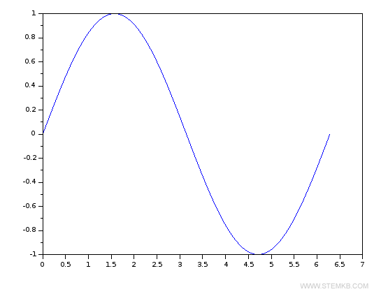
To illustrate, you can easily graph the sine function in the interval from 0 to 2*pi.

Create a vector of values for the independent variable x

--> x = linspace(0, 2*%pi, 100);

Calculate the corresponding values of the function y = sin(x)

--> y = sin(x);

Use the plot() function to draw the graph.

--> plot(x, y);

A new window will open displaying the graph of the function y = sin(x) in the specified interval.

This tutorial has shown you how to leverage the powerful mathematical features of Scilab for your computational needs.

As we continue to explore, you'll find Scilab is an invaluable tool in the world of numerical computation.