Creating NumPy arrays in Python

One of the best things about NumPy is that it lets you work with numbers, matrices, and vectors incredibly efficiently - much faster than using Python's standard lists.

What is a NumPy array? A NumPy array is essentially a data structure that can store a collection of elements (typically numbers, but it can also handle strings), arranged in rows and columns, just like a mathematical matrix. The key difference from Python’s lists is that NumPy is optimized for handling large amounts of numerical data with high efficiency.

Now, let’s see how to create an array.

First of all, make sure you’ve installed the NumPy package if you haven’t done so already. Then, you’ll need to import it in your Python code.

import numpy as np

Once imported, you can create both one-dimensional arrays (e.g., vectors) and multi-dimensional arrays (e.g., matrices, tensors, and more).

Creating a NumPy array

Let’s say you want to create a simple array containing the numbers 1 through 5.

With NumPy, you can do this in a very intuitive way using the array() method:

arr = np.array([1, 2, 3, 4, 5])
print(arr)

Just make sure to place the array elements inside square brackets, separated by commas.

Here’s the result:

[1 2 3 4 5]

That’s it! You’ve created a one-dimensional array, also known as a "vector".

The main advantage over Python lists is that a NumPy array is much faster when performing mathematical operations on large datasets.

Two-dimensional arrays: matrices

If you want to work with something more complex, like a matrix (a two-dimensional array), NumPy makes it easy:

matrix = np.array([ [1, 2, 3] , [4, 5, 6] , [7, 8, 9] ])
print(matrix)

In this case, you need to enclose each row of the matrix in square brackets, in addition to the outer brackets that enclose the entire matrix.

This will create a 3x3 matrix:

[[1 2 3]
[4 5 6]
[7 8 9]]

See how neat that looks? Each list inside the main list represents a row. And with this matrix, you can perform mathematical operations far more efficiently than with traditional Python lists.

Multidimensional Arrays

A multidimensional array is a data structure used to organize numbers across two or more dimensions.

Think of it as a list of lists, a table, or even a stack of tables layered one on top of the other.

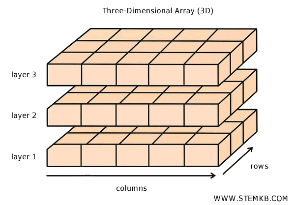
Here's an example of a 3-dimensional array. It consists of three matrices, each with 3 rows and 5 columns.

This kind of structure is essential when working with complex datasets - such as images, time series, scientific measurements, or large numerical tables.

NumPy is the core library for working with multidimensional arrays in Python. Let’s dive into what they are and how to use them, with a few hands-on examples.

One-Dimensional Array (1D)

A one-dimensional array is the simplest form: a single sequence of values, much like a basic Python list.

import numpy as np
np.random.seed(0)
x1 = np.random.randint(10, size=6)

This snippet generates six random integers between 0 and 9.

The line np.random.seed(0) sets the seed for the random number generator, ensuring that the results are reproducible every time the code runs.

The function np.random.randint(10, size=6) creates a 1D array containing six randomly selected integers from 0 to 9.

Here’s the resulting array assigned to x1:

array([5, 0, 3, 3, 7, 9])

You might think of this as a student’s scores from six different tests - all laid out in a single row.

Two-Dimensional Array (2D)

A two-dimensional array resembles a grid or matrix, consisting of rows and columns - similar to a spreadsheet.

x2 = np.random.randint(10, size=(3, 4))

This generates a 3×4 matrix filled with random integers between 0 and 9.

Here’s an example of what the output might look like:

array([[3, 5, 2, 4],
          [7, 6, 8, 8],
          [1, 6, 7, 7]])

You can think of this as a table where each row represents a student and each column corresponds to a subject.

In this case, it could represent report cards for 3 students, each evaluated across 4 subjects.

Three-Dimensional Array (3D)

For even more complex data, you can use a three-dimensional array - a stack of 2D arrays.

x3 = np.random.randint(10, size=(3, 4, 5))

This creates three separate 4×5 tables, forming a 3D array.

Here’s one possible output:

array([[[8, 8, 1, 6, 7],
[7, 8, 1, 5, 9],
[8, 9, 4, 3, 0],
[3, 5, 0, 2, 3]],

[[8, 1, 3, 3, 3],
[7, 0, 1, 9, 9],
[0, 4, 7, 3, 2],
[7, 2, 0, 0, 4]],

[[5, 5, 6, 8, 4],
[1, 4, 9, 8, 1],
[1, 7, 9, 9, 3],
[6, 7, 2, 0, 3]]])

How should you interpret this structure? Imagine you're collecting five different environmental readings (e.g. temperature, humidity, pressure, wind speed, and brightness) at four different times of day (morning, noon, afternoon, evening) over a span of three consecutive days.

• Each 2D block represents one day.
• Each row corresponds to a specific time of day.
• Each column represents one of the five measured variables.

It’s like having multiple Excel sheets in a single workbook, all following the same structure.

Why are multidimensional arrays so useful?

They allow you to store and structure data in a clean, organized way, which makes analysis much easier and more efficient.

Whether you're working with images (which are often 2D or 3D arrays), videos, scientific simulations, or just large numeric datasets, mastering multidimensional arrays unlocks powerful capabilities across a wide range of applications.

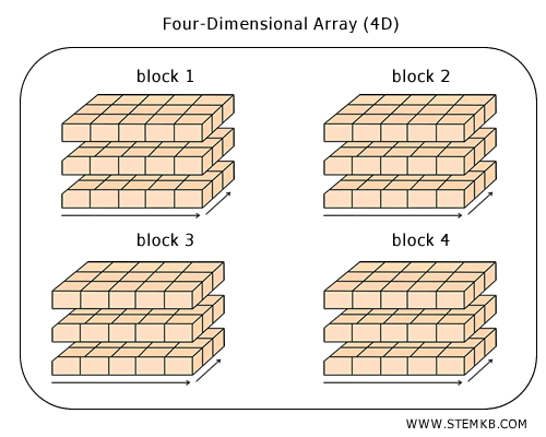
Are there arrays beyond three dimensions? Absolutely. While they're harder to visualize, NumPy can handle arrays with four, five, six, or even more dimensions. These high-dimensional arrays are commonly used in fields like image processing, scientific modeling, and complex data pipelines. They're especially valuable when working with large, structured datasets that need to be stored and accessed efficiently. For instance, you can think of a 4-dimensional array as a drawer containing multiple 3D arrays - each of which, in turn, holds a collection of 2D tables. Here's a way to visualize it:

Working with arrays

This is where NumPy really shines. Let’s say you want to add every element of one array to another array of the same shape. With NumPy, it’s incredibly straightforward.

For example, imagine you have these two arrays:

arr1 = np.array([1, 2, 3])
arr2 = np.array([4, 5, 6])

To add them, you just need to do this:

sum_array = arr1 + arr2
print(sum_array)

And here’s the result:

[5 7 9]

In algebraic terms, Python adds the elements of the two vectors that are in the same position.

$$ (1,2,3) + (4,5,6) = (1+4, 2+5, 3+6) = (5,7,9) $$

The same logic applies to all mathematical operations: multiplication, division, subtraction, and exponentiation.

For example, try multiplying the two arrays:

multiplication = arr1 * arr2
print(multiplication)

[ 4 10 18]

Notice how the operation happens element by element, multiplying the first element of `arr1` by the first element of `arr2`, and so on.

$$ (1,2,3) \cdot (4,5,6) = (1 \cdot 4, 2 \cdot 5, 3 \cdot 6) = (4,10,18) $$

But what about matrices?

When working with matrices, you have two types of multiplication at your disposal.

For example, let’s define two 2x2 matrices called 'matrix1' and 'matrix2':

matrix1 = np.array([[1, 2], [3, 4]])
matrix2 = np.array([[5, 6], [7, 8]])

In linear algebra, matrix multiplication is done using the row-by-column product.

To perform this, you can use the dot() method:

product = np.dot(matrix1, matrix2)
print(product)

[[19 22]
[43 50]]

Here, the np.dot function carries out the row-by-column product between the matrices, just as in linear algebra.

$$ \begin{pmatrix} 1 & 2 \\ 3 & 4 \end{pmatrix} \cdot \begin{pmatrix} 5 & 6 \\ 7 & 8 \end{pmatrix} = \begin{pmatrix} 1 \cdot 5 + 2 \cdot 7 & 1 \cdot 6 + 2 \cdot 8 \\ 3 \cdot 5 + 4 \cdot 7 & 3 \cdot 6 + 4 \cdot 8 \end{pmatrix} =  \begin{pmatrix} 19 & 22 \\ 43 & 50 \end{pmatrix} $$

If, on the other hand, you want to perform an element-wise multiplication (also known as the "Hadamard product"), you can simply use the `*` operator:

hadamard = matrix1 * matrix2
print(hadamard)

[[ 5 12]
[21 32]]

In this case, the multiplication occurs between the corresponding elements of the two matrices.

$$ \begin{pmatrix} 1 & 2 \\ 3 & 4 \end{pmatrix} \cdot \begin{pmatrix} 5 & 6 \\ 7 & 8 \end{pmatrix} = \begin{pmatrix} 1 \cdot 5 & 2 \cdot 6 \\ 3 \cdot 7 & 4 \cdot 8 \end{pmatrix} = \begin{pmatrix} 5 & 12  \\ 21 & 32 \end{pmatrix} $$

As you can see, NumPy is incredibly powerful. It allows you to perform mathematical operations on arrays and matrices in a way that’s both efficient and easy to read. And we’re just scratching the surface! You can do so much more, like calculating eigenvalues, inverting matrices, solving systems of equations... In short, NumPy is an essential tool for working with linear algebra in Python.