Standard Deviation
Standard deviation is a statistical measure that shows how much data points in a set vary from the average, helping us understand the uncertainty in the data. It’s calculated as the square root of the average of the squared differences between each data point and the mean.
$$ \sigma = \sqrt{\frac{(x_1 - \bar{x})^2 + (x_2 - \bar{x})^2 + \ldots + (x_N - \bar{x})^2}{N}} $$
Here, \( x_i \) represents each measurement, \( \bar{x} \) is the mean, and \( N \) is the total number of measurements.
When dealing with a large set of experimental measurements, the standard deviation gives a clearer view of the uncertainty.
This metric tells us how closely the values cluster around the mean: the smaller it is, the more precise the measurements.
An Example
Suppose you have five time measurements (in seconds) taken during an experiment.
$$ 20.5, \ 21.0, \ 21.5, \ 22.0, \ 20.0 \ s $$
Using the range method to estimate absolute error, you would simply consider the extremes:
$$ e_x = \frac{22.0-20.0}{2} = 1 \ s $$
This method, however, doesn’t account for all measurements, so it’s fairly approximate.
To get a more accurate sense of uncertainty, you can calculate the standard deviation.
First, calculate the mean (\(\bar{x}\)) of the measurements.
$$ \bar{x} = \frac{20.5 + 21.0 + 21.5 + 22.0 + 20.0}{5} = \frac{105.0}{5} = 21.0 \, \text{seconds} $$
Next, find the deviation of each measurement from the mean by subtracting the mean from each measurement:
- \(20.5 - 21.0 = -0.5\)
- \(21.0 - 21.0 = 0.0\)
- \(21.5 - 21.0 = 0.5\)
- \(22.0 - 21.0 = 1.0\)
- \(20.0 - 21.0 = -1.0\)
These deviations are: \(-0.5, 0.0, 0.5, 1.0, -1.0\).
Note that if we took the average of these deviations, we’d get zero because the positive and negative deviations cancel each other out. $$ \frac{(-0.5)+0.0+0.5+1.0+(-1.0)}{5} = \frac{0}{5} $$ To avoid this, we square each deviation, making them all positive, and then calculate the average of these squares. Finally, we take the square root to bring the standard deviation back to the original unit of measurement.
Square each deviation to remove the negative signs.
- \((-0.5)^2 = 0.25\)
- \((0.0)^2 = 0.0\)
- \((0.5)^2 = 0.25\)
- \((1.0)^2 = 1.0\)
- \((-1.0)^2 = 1.0\)
The squared deviations are therefore: \(0.25, 0.0, 0.25, 1.0, 1.0\).
Add these values together and divide by the number of measurements (5) to get the average of the squared deviations.
$$ \text{average of squared deviations} = \frac{0.25 + 0.0 + 0.25 + 1.0 + 1.0}{5} = \frac{2.5}{5} = 0.5 $$
Finally, to obtain the standard deviation (σ), take the square root of the average of the squared deviations.
$$ \sigma = \sqrt{0.5} \approx 0.71 \, \text{seconds} $$
The result, \( \sigma \approx 0.71 \) seconds, represents the standard deviation for this set of measurements.
$$ x = \bar{x} \pm \sigma $$
In this case, the mean is \( \bar{x} = 21 \ s \) and \( \sigma = 0.71 \ s \).
$$ x = 21.0 \pm 0.71 \ \text{sec} $$
This result gives a more precise indication of how closely the measurements cluster around the mean of \(21.0\) seconds.
The lower the standard deviation, the closer the measurements are to the mean, indicating higher accuracy.
The standard deviation is not only a measure of uncertainty but also a key tool in applying the Gaussian curve to data representation. It allows us to predict the likelihood of values clustering around the mean in a normal distribution.
The Gaussian Curve and Normal Distribution
In statistics, when we gather a large enough number of measurements that are subject to random errors, these values tend to follow a specific shape called the Gaussian curve or normal distribution.
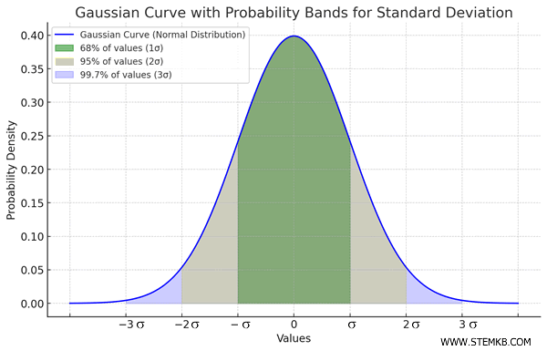
The Gaussian curve, or "bell curve," is symmetric around the mean and describes the probability of obtaining a measurement within a certain range of the mean.

In a normal distribution:
- About 68% of values fall within one standard deviation (σ) of the mean,
- Approximately 95% fall within two standard deviations,
- Roughly 99.7% fall within three standard deviations.
This characteristic makes the Gaussian curve a universal model for describing uncertainty across a wide range of natural and experimental phenomena, from physics and biology to economics.
Example. Suppose you have a mean of 20.5 seconds and a standard deviation of 0.3 seconds, across 1,000 measurements. With this data, you can estimate that:
- 68% of the values fall within one standard deviation (σ) of the mean, so around 680 measurements are between 20.2 and 20.8 seconds.
- 95% of values lie within two standard deviations (2σ) of the mean, meaning about 950 measurements are between 19.9 and 21.1 seconds.
- 99.7% of values fall within three standard deviations (3σ) of the mean, with around 997 measurements between 19.6 and 21.4 seconds.
These ranges represent the expected distribution of measurements around the mean, with each standard deviation level covering more of the data.
In this way, standard deviation is not just a mathematical concept but a powerful tool for interpreting data distribution around the mean.

