
Linearly Dependent Quantities
In physics, many natural phenomena can be described using mathematical relationships. Among these, linearly dependent quantities stand out as particularly significant, connected by a simple yet powerful equation:
\[ y = kx + y_0 \]
This linear equation establishes a direct and predictable relationship between two physical quantities.
It serves as an essential tool for understanding and analyzing a wide variety of systems, from uniform linear motion to the operation of electrical circuits.
The Linear Relationship
The equation \( y = kx + y_0 \) defines a linear dependency between two variables: \( x \) and \( y \). Here’s what its components signify:
- \( k \) is the slope or gradient of the line. It indicates how \( y \) changes in response to variations in \( x \). For instance, in a directly proportional relationship, \( k \) represents the constant rate of change.
- \( y_0 \) is the y-intercept, representing the value of \( y \) when \( x = 0 \). This term shifts the line vertically on the Cartesian plane.
- \( x \) and \( y \) are the physical quantities being related. Typically, \( x \) is the independent variable, while \( y \) is the dependent one.
A practical example is uniform linear motion, where an object’s position (\( s \)) changes linearly with time (\( t \)):
\[ s = vt + s_0 \]
In this equation, \( v \) represents the constant velocity, \( t \) is the time, and \( s_0 \) is the initial position.
A Concrete Example
One of the most well-known applications of linear dependence is Ohm’s Law in electrical circuits.
This law states that the voltage (\( V \)) across a conductor is directly proportional to the current (\( I \)) flowing through it, with the resistance (\( R \)) serving as the proportionality constant:
$$ V = RI $$
In this case, the slope is \( k = R \), and the y-intercept is zero (\( y_0 = 0 \)), reflecting a direct proportionality with no offset.
The simplicity of this relationship is one of its strengths: knowing any two of the three variables allows you to determine the third.
Other Practical Examples. Physics provides numerous other examples of linear dependencies between quantities. For instance, in Hooke’s Law, the force (\( F \)) exerted by a spring is proportional to its extension (\( x \)): $$ F = kx $$ This is just one of many such examples.
Example 2
Consider the linear relationship \( y = 2x + 3 \), where \( k = 2 \) is the slope, and \( y_0 = 3 \) is the y-intercept.
$$ y = 2x + 3 $$
We can calculate \( y \) for various values of \( x \), such as from 0 to 10.
Here’s a table illustrating the \( x \)-values and their corresponding \( y \)-values based on the equation \( y = 2x + 3 \).
| x | y |
|---|---|
| 0 | 3 |
| 1 | 5 |
| 2 | 7 |
| 3 | 9 |
| 4 | 11 |
| 5 | 13 |
| 6 | 15 |
| 7 | 17 |
| 8 | 19 |
| 9 | 21 |
| 10 | 23 |
Each increase in \( x \) by one unit leads to a constant increase in \( y \) by 2, which is the slope (\( k \)).
On a graph, the points align perfectly along a straight line.
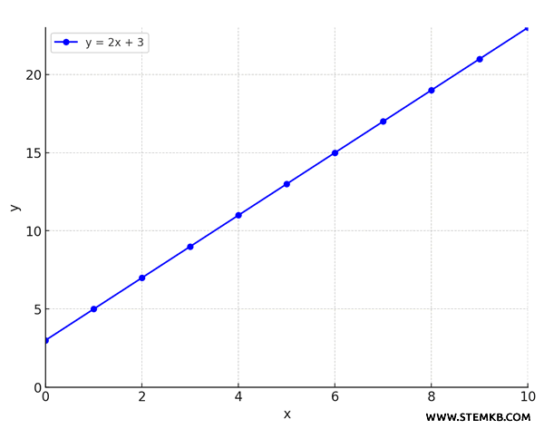
This visual representation reinforces the linear nature of the relationship.
The Advantages of Linearity
Linear relationships are fundamental because they make equations straightforward to solve and outcomes predictable.
Once \( k \) and \( y_0 \) are known, \( y \) can be calculated for any given \( x \).
This clarity and simplicity allow us to model complex systems and make accurate predictions.
Linearity often serves as the foundation for more advanced analysis, providing a reliable starting point for developing intricate models. By viewing the world through the lens of these relationships, we can uncover order and consistency even in seemingly chaotic phenomena.


