Creating Polar Plots in Matlab

In this lesson, I'll explain how to create a polar plot in Matlab.

What is a polar plot? You see, polar plots are these charming circular graphs that display data using their polar coordinates. They're quite popular in the scientific arena, and they have a certain elegance about them.

Let me demonstrate with a hands-on example.

First, we need to create an array called 'theta' to hold our angular variations:

>> theta = 0 : 0.1 : 2*pi;

This little command crafts an array ranging from 0 to 2π (that's 360°) in increments of 0.1.

Next, we'll define another array, 'y1,' with the function y1 values corresponding to each angular variation in theta:

>> y1=0.5+(1.3).^(theta);

Now, 'y1' represents the codomain of our function, while 'theta' takes care of the domain.

Thus, the arrays theta and y1 have the same number of elements.

With our arrays in place, we can move on to the exciting part - constructing the polar plot. Simply type the Polar() function like so:

>> PolarGraph = polar(theta,y1,"*");

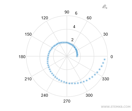
And there you have it! Matlab will gracefully display the behavior of function y1 using its polar coordinates.

In our case, we've managed to create a mesmerizing spiral function.

But wait, there's more! What if we want to display two functions in a single polar plot?

Let's clear the screen with 'clf' to start fresh and recreate the 'theta' array with the same angular variations.

clf

Then, we create the array theta again with the angular variations (domain of the function):

>> theta = 0 : 0.1 : 2*pi;

Now, we'll generate two new arrays, 'y1' and 'y2,' for two distinct functions that vary with theta:

>> y1=0.5+(1.3).^(theta);
>> y2 = 3*(1 - cos(theta));

Combine the two functions within a matrix [m]

>> m = [y1;y2];

Finally, use the Polarplot() function to create the polar plot:

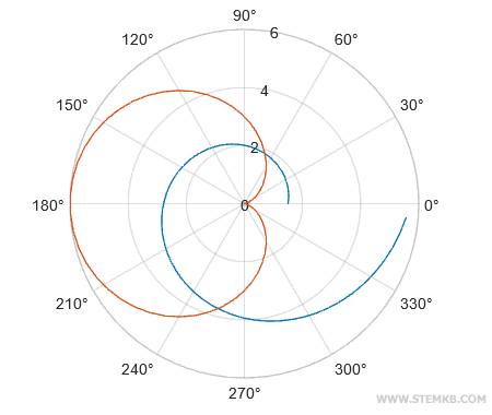
>> PolarGraph = polarplot(theta,m);

Both functions are displayed in the polar plot.

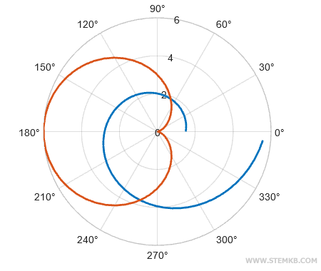
To thicken the plot lines, apply the set() function.

set(PolarGraph,"LineWidth",2);

And just like that, we've doubled the line thickness.

To further embellish our masterpiece, let's add a legend using the legend() function.

legend("y1","y2");

The legend box now tastefully adorns the edge of our graph.

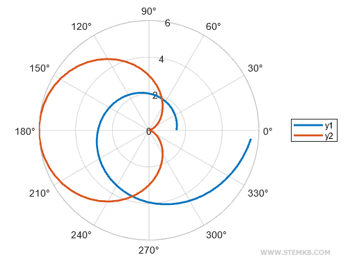
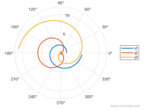
Remember, this technique isn't limited to just two functions. You can represent three or more functions in a single polar plot by following the same procedure. Define additional functions, create a matrix with all the functions, and use the polarplot(theta, m) function to display the overlapping graphs. The result is a captivating polar plot featuring multiple functions, all vying for your attention. For example, define another function y3 = 0.7 - (1.9).*theta in addition to y1 and y2. Then, create a matrix with three functions m = [y1; y2; y3]. Finally, use the function polarplot(theta, m) to display the three overlapping graphs in the same polar plot. Now, the polar plot displays three overlapping functions.

Now the polar plot displays three functions.