Graph Theory in Python

This tutorial dives into working with graphs in Python using the NetworkX module, showcasing its power for dealing with complex network structures and dynamics.

What is NetworkX? It's a robust Python library designed for the creation, manipulation, and exploration of the structure, dynamics, and functions of complex networks.

Let's walk through a straightforward example to construct a graph, add nodes and edges, and then visualize our creation.

Ensure you have NetworkX and Matplotlib installed in your Python setup before proceeding. These installations can be done through the pip command from your computer's command line:

pip install networkx matplotlib

The "matplotlib" module is essential for rendering graphs visually.

If you're working within an Integrated Development Environment (IDE) like PyCharm, handling modules and external libraries becomes more streamlined thanks to the built-in tools and features. Follow your IDE's guidelines to incorporate new modules into your Python environment seamlessly.

With the necessary modules installed, you can import them into your script with the import command.

import networkx as nx
import matplotlib.pyplot as plt

Now, you have access to the full suite of NetworkX functionalities.

Start by creating a graph object with the Graph() function.

G = nx.Graph()

Add nodes to your graph using add_node(), and for adding multiple nodes simultaneously, utilize add_nodes_from().

G.add_node(1)
G.add_nodes_from([2, 3, 4, 5])

With five vertices added, you're ready to connect them using edges with the add_edge() function, and add_edges_from() for multiple edges.

G.add_edge(1, 2)
G.add_edges_from([(2, 3), (3, 4), (4, 5), (1, 5)])

Edges automatically bring into existence any nodes not previously added.

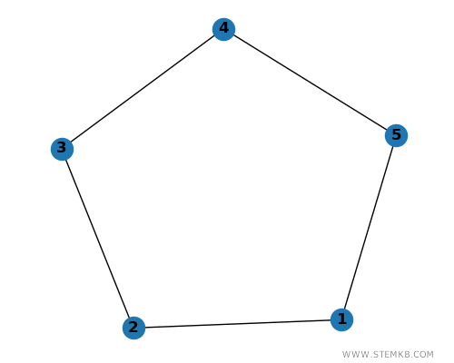
Visualize your graph with nx.draw(), which produces a graphical representation of your network.

nx.draw(G, with_labels=True, font_weight='bold')

The "with_labels=True" option labels your nodes within the graph. Bring it to life on the screen with matplotlib's show() method.

plt.show()

You've now created an undirected graph, labeling each vertex with identifiers, a testament to NetworkX's flexibility to accommodate various graph types, including weighted, directed (digraphs), and multigraphs.

NetworkX also boasts a comprehensive suite of algorithms for network analysis.

Creating a Directed Graph

To craft a directed graph, or DiGraph, you'll start by creating a DiGraph object.

What's a Directed Graph? It's a network of nodes linked by edges with directions that specify the flow from one node to another, establishing a clear path through the network.

Here's how to set up a directed graph with NetworkX, demonstrating node and edge addition, and visualization:

import networkx as nx
import matplotlib.pyplot as plt

# Creating a DiGraph object
G = nx.DiGraph()

# Adding nodes
G.add_node(1)
G.add_nodes_from([2, 3, 4, 5])

# Adding directed edges
G.add_edge(1, 2)
G.add_edges_from([(2, 3), (3, 4), (4, 5), (5, 1)])

# Visualizing the DiGraph
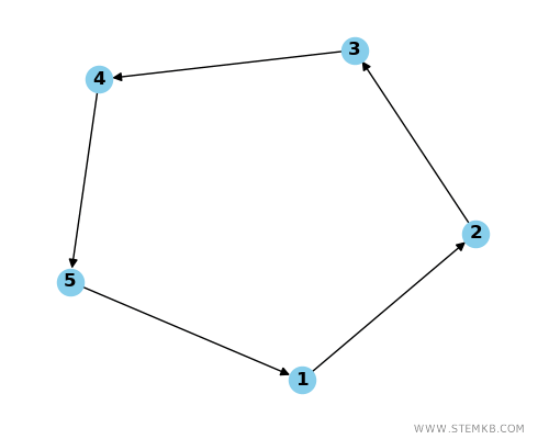
nx.draw(G, with_labels=True, font_weight='bold', node_color='skyblue', arrowstyle='-|>', arrowsize=12)
plt.show()

Choosing DiGraph signifies the creation of a directed graph, where the directionality of each edge is clearly defined, showcasing the flow from one node to another.

The visual representation is enhanced with arrow styles and sizes, making the directional paths between nodes evident.

This tutorial has guided you through generating both an undirected graph and a directed