Matlab's polyfit() function

Let me tell you about this nifty little function in Matlab called polyfit(). You can use it to find a polynomial that fits a series of data.

polyfit(Y)

The argument of the function is an array containing the data.

For instance, consider the following set of data:

>> X = [ 1 2 3 4 5 6 ]
>> Y = [ 3 8 6 9 7 8 ]

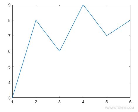
You can represent this series of data with a plot using the function plot(X,Y).

>> plot(X,Y)

It produces the following graph:

Then, if you want to find a first-degree polynomial that fits this data, you simply use the polyfit(X,Y,1) function, which will give you the coefficients of the first-degree polynomial.

>> P = polyfit(X,Y,1)

The result is:

P =
0.71429 4.33333

These are the coefficients of the first-degree polynomial:

$$ P_1(x) = 0.71429 \cdot x + 4.33333 $$

You can calculate the values of the polynomial for each element of the X array using the polyval() function, which takes as argument the coefficients of the polynomial and the array X.

>> polyval(P,X)

This function calculates the values of the polynomial for every element of the X array, and the result is:

ans =
5.0476 5.7619 6.4762 7.1905 7.9048 8.6190

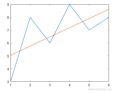
Finally, you can display both the data and the polynomial on a Cartesian plane using the plot() function.

plot(X,Y,X,polyval(P,X))

The first-degree polynomial (linear) finds a line that approximates the data series.

Example 2

Now, suppose you want to find a second-degree polynomial that fits the data.

You can use the same functions, but with the argument 2 instead of 1 in the polyfit() function.

>> P = polyfit(X,Y,2)

This will give you the coefficients of the second-degree polynomial, which you can use with the polyval() function to calculate the values of the polynomial for each element of the X array.

P =
-0.35714 3.21429 1.00000

These are the coefficients of the second-degree polynomial.

$$ P_2(x) = -0.35714 \cdot x^2 + 3.21429 x + 1.0 $$

Now, you can calculate the values of the polynomial using the polyval(P,X) function.

>> polyval(P,X)

The result is an array with the values of the polynomial for each element of the X array.

ans =
3.8571 6.0000 7.4286 8.1429 8.1429 7.4286

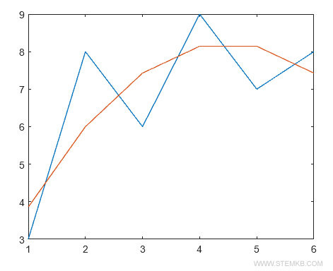
Once again, you can display both the data and the polynomial on a Cartesian plane using the plot() function.

plot(X,Y,X,polyval(P,X))

The second-degree polynomial (red line) fits the data series better.

Example 3

Finally, you can repeat the same process to find a third-degree polynomial that fits the data.

>> P = polyfit(X,Y,3)

The result of the function is:

P =
0.18519 -2.30159 9.08466 -3.66667

These are the coefficients of the third-degree polynomial.

$$ P_3(x) = 0.18519x^3 -2.30159 \cdot x^2 + 9.08466 x - 3.66667 $$

You can calculate the values of the polynomial using the polyval(P,X) function.

>> polyval(P,X)

This function produces the values of the polynomial for every element of the X array.

ans =
3.3016 6.7778 7.8730 7.6984 7.3651 7.9841

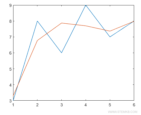
Now, you can visualize both graphs on the Cartesian diagram using the plot() function.

plot(X,Y,X,polyval(P,X))

The third-degree polynomial (red line) approximates the data series even better.

As you increase the degree of the polynomial, the approximation error decreases, because the polynomial better fits the series of data. So there you have it, a handy tool to find the best polynomial to fit your data in Matlab.